About

Before we can dive into multi-spectral satellite images, I think a quick refresher on how images are encoded and represented in memory is a good starting point.

Binary encoding

Let's take a short recap of how classical computer vision images are encoded in memory. Internally a computer (ignoring quantum-computing) only works with binary numbers. A binary number is either a 0 or a 1, on or off. The value of such a binary number is called a bit. The smallest data-element is called a byte. A byte consists of 8 bits. There are different ways how we could use these 8 bits/1 byte to encode our data. The data we are trying to store/load defines how we interpret the data. If we want to only work with positive integers, we use an unsigned integer type. An unsigned integer with 8 bits can encode all numbers from 0$-$255. If all bits are 1, also called set, the value is 255. If all bits are 0 the corresponding value is 0.¹

Grayscale images

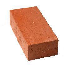
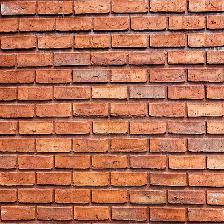
Images, like everything in a computer, are also only encoded in binary values. The most straightforward images are grayscale images. The possible colors of each pixel of a grayscale image can only range from black to gray to white, with all different gray shades in-between. Pixels are the basic elements of a picture. The word itself, pixel, is a combination of the words picture and element/cell. So an image consists of pixels, similar to how a brick wall consists of bricks.

We can understand how simple 8-bit grayscale images are encoded with the knowledge of our previous simple encoding scheme. The 8-bit refers to the color-depth. It indicates how many bits are used per channel. We only have a single channel for a grayscale image, the colors range from black to white. (We will take a closer look at different channels in the next post.) For now, we note that our grayscale channel is encoded with 8-bits. Or, put differently, we use 8-bits for every pixel to show different shades of gray. With 8-bits, we can color each pixel in 256 (2⁸) different ways.

With the numpy and PIL library, we can easily create our own 8-bit grayscale image by merely changing the value of a byte.

import numpy as np
from PIL import Image, ImageOps

def to_grayscale_image(x):
    grayscale_8_bit_mode = "L"
    return Image.fromarray(x, mode=grayscale_8_bit_mode)

def upscale_image(img, img_width=224, img_height=224):
    return img.resize((img_width, img_height), resample=Image.NEAREST)

# PIL requires np arrays as input
# Datatype is uint8, our unsigned int consisting of 8-bits
# zero is our single byte/value with value 0
# -> Array has a width and height of 1
zero = np.zeros((1, 1), dtype=np.uint8)

img_values = {
    "pixel_0": zero, 
    "pixel_64": zero + 64, 
    "pixel_192": zero + 192, 
    "pixel_255": zero + 255
}

for name, value in img_values.items():
    img = to_grayscale_image(value)
    img = upscale_image(img)
    bordered_img = ImageOps.expand(img, border=1, fill="black")
    # display(bordered_img) # To display in jupyter
    bordered_img.save(f"2020-09-02/{name}.png")

You can also play around with the following widget to see the grayscale values of your own choice²:

Until now, we did not care about the resolution of our images. The resolution defines how many pixels we use to visualize the object. A resolution of 1 corresponds to a single pixel. But, with a single-pixel picture, we cannot retain a lot of information. As shown above, we could only create a single shade of gray. Let's increase our resolution for the following images to a size of 224 pixels x 224 pixels. With more pixels, we can show more levels of detail.

Now we can extend our previous code to draw gradients!

zeros = np.zeros((224, 224), dtype=np.uint8)
x_gradient = np.arange(0, 224, dtype=np.uint8).reshape(1, 224)
y_gradient = np.arange(0, 224, dtype=np.uint8).reshape(224, 1)

# Using numpy's broadcasting
x_grad_2d = zeros + x_gradient
y_grad_2d = zeros + y_gradient
sum_grad_2d = x_gradient + y_gradient
diff_grad_2d = x_gradient - y_gradient

# Convert to a grayscale image as before
# and save or show files

Visualization of different 8-bit grayscale images

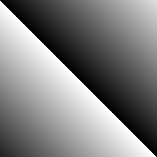
If we don't limit ourselves to simple mathematical operations, we can show images with great detail.

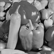
The pepper's image consists of the following values. Each value is saved as a single byte on disk.

array([[ 71,  96,  92, ..., 136, 132, 127],
       [ 87, 119, 113, ..., 181, 176, 170],
       [ 83, 114, 111, ..., 178, 174, 166],
       ...,
       [ 92, 120, 108, ..., 191, 198, 198],
       [ 88, 124, 104, ..., 202, 198, 194],
       [ 78, 126, 106, ..., 200, 193, 188]], dtype=uint8)

Important: Even if these images reveal a lot of information to us humans, in the end, they are only stored as 0s and 1s on the computer.

Before we move with the next topic, let's review what we have learned so far.

Summary

Increasing the number of pixels (resolution) allows us to encode more details. The color-depth shows us how many bits we use per channel to encode a color. Our previous 8-bit grayscale pixel can, therefore, encode 256 different shades of gray. With a higher color-depth, we have access to more shades. But what is when we want to enrich our image with colors?

How to add colors to our image and how remote sensing images are different will be the topic of the next blog post!

Until then, have a productive time!

1. A quick refresher on how to translate binary numbers to unsigned integers can be found on ryanstutorials ↩

2. Sometimes the initialization of the widgets hang. The best solution I found was reopening the same page in Incognito Mode and reloading the page. It can take up to a minute until the widgets are loaded.↩