Introduction to the BigEarthNet dataset
A look at the new BigEarthNet dataset, based on sentinel-2 multispectral images.


About
In the previous post, understanding spectral reflectance, we saw that objects could be differentiated by their surface reflectance. The surface reflectance can be sensed as multi-spectral images from satellites. In the following post, we will examine the Sentinel-2 mission and the resulting data. Afterwards, we will review an example remote sensing dataset, BigEarthNet.
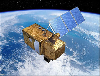
Sentinel-2 mission
Sentinel-2 is an earth-observation mission and consists of two satellites Sentinel-2A and Sentinel-2B. Both of which are operated by the European Space Agency (ESA). The task is to gather multi-spectral data for climate change, agriculture monitoring, and emergency management. The data is published under a free and open data policy, making it valuable for academic purposes.
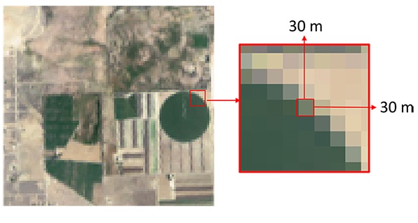
With both satellites and their large field of view (290km), they can sense most of the earth's land cover every 5 days. The revisit frequency is also called the temporal resolution. The spatial resolution is reported as $XX\,\text{m}$, which refers to the length and height of a pixel. So a resolution of 10m would correspond to a single pixel capturing an area of 10m x 10m, or 100m². An example remote sensing image can be seen in the following figure. The Sentinel-2 satellites have a spatial resolution of 10m (four visible and near-infrared), 20m (six red edge and short-wave infrared), and 60m (three atmospheric correction) bands. [1]
In total, thirteen bands are sensed, ranging from the visible/near-infrared (VNIR) to the short-wave infrared (SWIR) spectrum. Each band has effectively 16-bits per channel, or as it is commonly referred to in the remote image sensing community, a radiometric resolution of 16-bits. The term radiometric resolution highlights the domain in which the images are used but is no different from bits per channel1.
The following figure shows all thirteen bands grouped by their spatial resolution. ESA introduced Band 8A in the Sentinel-2 mission as band 08 was too contaminated by water vapor and insensitive to other parameters for some applications. But, the original sensor for band 08 remained in the sensory equipment. The narrowness of band 8A should make the results less noisy towards water vapor but still be wide enough for most applications [2].
alt.Chart(sentinel_band_data).mark_rect().encode(
    x=alt.X("start:Q", title="Wavelength in nm"),
    x2="end:Q",
#     color=alt.Color("Band", scale=alt.Scale(scheme="category20")),
    color=alt.Color("Color", scale=None),
    tooltip=[
        alt.Tooltip("Band:O", title="Band"),
        alt.Tooltip("Usage"),
        alt.Tooltip("Central Wavelength"),
        alt.Tooltip("Spatial Resolution"),
    ]
).transform_calculate(
    start="datum['Central Wavelength'] - 1/2 * datum['Bandwidth']",
    end="datum['Central Wavelength'] + 1/2 * datum['Bandwidth']"
).properties(
    height=100,
    width=600
).facet(
    row="Spatial Resolution"
)
Everyone can register on scihub.copernicus.eu and search for remote sensing imagery. The images, also called tiles or granules, from the Sentinel-2 mission sense an area of 100km² and are ~600MB in size. [3] The Copernicus program provides two types of data for public usage:
- L2A (Level 2A with atmospheric correction)
- L1C (Level 1C without atmospheric correction)
Applying atmospheric correction algorithms transform a so-called TOA (Top Of Atmosphere) to a BOA (Bottom Of Atmosphere) image. If one is interested in the surface reflectance values, or more generally on the objects on the ground, the L2A data should be preferred. In the case of missing L2A data, the Sentinel-2 toolbox can be used to generate L2A from L1C images.
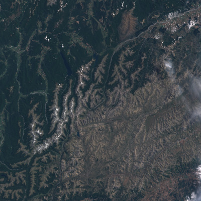
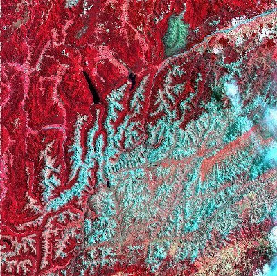
Fig. 2a shows the visible bands of a randomly selected image with low cloud coverage. Remote sensing images that show the visible bands, like classic RGB images are called true-color images (TCI). To visualize the data from the other bands one can:
- Show each band independently as a grayscale image
- Map three bands to the classic RGB channels of an image (called false-color image/composite)
Fig. 2b shows a popular false-color composite, using the bands 08, 04, and 03. With the band in the near-infrared spectrum (band 08) as the red channel, the healthy green vegetation will light up in bright red. As the bare soil has a low reflectance in the near-infrared spectrum, it will range from tan to turquoise. With the EO Browser, you can interact with satellite imagery and false-color composites without requiring you to download any images or manually applying transformations on different spectral bands.
To get most of the high-volume data from remote sensing images, one can employ deep-learning. Deep-learning has become the state-of-the-art solution to complex computer vision applications. Usually, deep-learning models are used on classic RGB images, but they also seem to be promising for these multi-spectral images. To train and test these models, researchers need large, high-quality datasets. The data assembly was not a problem, thanks to the open data policy of the Sentinel-2 imagery. Sumbul et. al [4] were able to assemble and published such a dataset, BigEarthNet.
BigEarthNet
The BigEarthNet archive uses Sentinel-2 tiles that are distributed over 10 countries from Europe 2. Only tiles with a cloud cover percentage under 1% containing no missing/faulty pixels were considered. The tiles were then split into smaller non-overlapping patches for further processing and publication. In total, the dataset consists of 590,326 patches, each of which covers a region of 1.200m x 1.200m. Due to the different spatial resolution of the various bands, the patches have different sizes. 120 x 120 pixels for 10m bands, 60 x 60 pixels for 20m bands, and 20 x 20 pixels for 60m bands.
As the archive is based on Sentinel-2 images, the radiometric resolution is 16-bits. The time-frame for the acquisition dates were between June 2017 $-$ June 2018. Due to the winter months generally having higher cloud coverages, the winter season has the fewest samples, as seen in the following chart.
season_data = pd.DataFrame([
    {"Season": "Autumn", "# Images": 154_943},
    {"Season": "Winter", "# Images": 117_156},
    {"Season": "Spring", "# Images": 189_276},
    {"Season": "Summer", "# Images": 128_951},
])

alt.Chart(season_data).mark_bar().encode(
    x="Season",
    y="# Images",
    tooltip=[
        alt.Tooltip("Season"),
        alt.Tooltip("# Images"),
    ],
).properties(
    width=300
)
The authors identified 70,987 patches that are fully covered by clouds, cloud shadows, and seasonal snow. They provide CSV files to exclude these patches if desired and recommend to do so if neural networks are only trained on the BigEarthNet dataset.
The last point to note is that not all bands are used in this dataset; band 10 is omitted. Band 10 does not include any surface-level information, as it is mainly used to detect cirrus clouds [5]. These clouds form at high altitudes and are transparent or semi-transparent in the optical bands but have a high impact on the original spectral reflectance [6]. For the data preprocessing step, the 10th band is a significant indicator of the data quality but does not hold any information for down-stream processes. To use the correct terminology, band 10 is important for TOA analysis and the conversion from TOA to BOA images. However, the other 60m bands used for atmospheric correction were not removed.
With that said, we have covered all the essential details of the BigEarthNet archive. But, before we move on and use the dataset, let's take a short recap.
Summary
The most important features of the Sentinel-2 earth-observation mission are:
- 2 satellites (Sentinel-2A/Sentinel-2B)
- Temporal resolution of 5 days
- Spatial resolution of 10m, 20m, and 30m (depending on the specific band)
- Radiometric resolution of 16-bits
- Senses 13 bands, from the visible/near-infrared to the short-wave infrared spectrum
- Open data policy
Thanks to the open data policy, researchers were able to create BigEarthNet, a large, freely available multi-spectral dataset for deep-learning. The significant properties are:
- Provides ~590,000 patches
- Each patch covers a region of 1.200m x 1.200m
- Various resolutions defined by Sentinel-2 specs
- Does not include band 10, as it does not contain surface-level information
- Provides CSV with all uninformative patches (patch with only snow/clouds)
References
- [1]European Space Agency, “Sentinel-2 spatial resolution.” 12-Oct-2020 [Online]. Available at: https://sentinel.esa.int/web/sentinel/user-guides/sentinel-2-msi/resolutions/spatial
- [2]European Space Agency, “Sentinel-2 Heritage.” 12-Oct-2020 [Online]. Available at: https://sentinel.esa.int/web/sentinel/missions/sentinel-2/heritage
- [3]European Space Agency, “Sentinel-2 Data Products.” 12-Oct-2020 [Online]. Available at: https://sentinel.esa.int/web/sentinel/user-guides/sentinel-2-msi/product-types
- [4]G. Sumbul, M. Charfuelan, B. Demir, and V. Markl, “Bigearthnet: A Large-Scale Benchmark Archive for Remote Sensing Image Understanding,” in IEEE International Geoscience and Remote Sensing Symposium, 2019 [Online]. Available at: http://bigearth.net/static/documents/BigEarthNet_IGARSS_2019.pdf
- [5]European Space Agency, “Sentinel-2 cloud masks.” 12-Oct-2020 [Online]. Available at: https://sentinel.esa.int/web/sentinel/technical-guides/sentinel-2-msi/level-1c/cloud-masks
- [6]S. Qiu, Z. Zhu, and C. E. Woodcock, “Cirrus clouds that adversely affect Landsat 8 images: What are they and how to detect them?,” Remote Sensing of Environment, no. Q, Sep. 2020 [Online]. Available at: https://www.sciencedirect.com/science/article/pii/S0034425720302546
1. There is some ambiguity of the actual radiometric resolution. The official website writes a radiometric resolution of 12-bits per channel, but the information is out of date. Inspection of images starting around 2016 reveals a resolution of at least 15-bits. But the full 16-bit range is used to encode special values. As the data will always end-up using 2 Bytes for storage (16-bits), it is commonly treated as a 16-bit image. I tried my best to comprehend the data range fully, but there are still some open questions. I am trying to answer these questions and have an open discussion on gis.stackexchange.com. Feel free to join the discussion!↩
2. These 10 countries are: Austria, Belgium, Finland, Ireland, Kosovo, Lithuania, Luxembourg, Portugal, Serbia, Switzerland↩